First, Let's try to understand what actually is “Constrained Random verification”.

As chip designs get more complex day by day, Traditional verification methods started failing the main verification objective of catching bugs.
This is because it is nearly impossible to simulate all the permutations and combinations of the inputs because of the time-market frame and resource utilization etc. This is when Constrained Random verification started gaining attention.

Let's take an example of a 5:7 decoder, which is going to be our DUT(Design Under Test). Now let's say we try to do the testing in the traditional method using a testbench, we will have to test out all the possible cases (that is 2⁵ = 32 combinations) to make sure that there are no bugs in the design.It will be a little tedious to test them all.

Here is where the concept of “constrained random verification” comes in handy.

This concept will allow us to generate random inputs. For 32 combinations it wouldn’t matter as its trivial but when it comes to 1000’s sequences in the case of SoC’s/ASIC, we can’t afford to do all the sequences, we can’t just blindly randomize everything hence the concept of “Constrained” to cover all the corner cases, which gives us more confidence.

With the below RTL design of the 5:7 decoder, we are assigning whenever an invalid input(Data_in) is given - we get a 0 at all the output ports else the valid cases.

Verification of circuit design takes place by comparing the desired result with passing the test input to the DUT. But, if we observe we have only 7 valid test cases rest are invalid, so constraining and checking randomly is more efficient to get a confirmation of the design’s functionality.

module decoder5to7(

input [5:0] Data_in,  // inputs

output reg [6:0] Data_out // outputs

);

//Whenever there is a change in the Data_in, execute the always block.

always @(Data_in)

case (Data_in)

5'b00000 : Data_out = 7'b0000001;

5'b01001 : Data_out = 7'b0000010;

5'b10010 : Data_out = 7'b0000100;

5'b00011 : Data_out = 7'b0001000;

5'b10100 : Data_out = 7'b0010000;

5'b01101 : Data_out = 7'b0100000;

5'b10110 : Data_out = 7'b1000000;

//To make sure that latches are not created.

default : Data_out = 7'b0000000;

endcase

endmodule

A 5:7 decoder is simple and just requires hardly a few minutes to test its functionality. Think of some complex circuits like finite state machines that do some complex task or 32-bit adders, which require many test cases to be tested upon. Manually verifying the logic by giving a set of inputs and comparing it with the expected one is tedious in this case because there are many different cases to test on with a lot of input bits, and even if we randomize we have a lot of cases to consider which is again time-consuming, so constraining the randomized inputs and checking for critical corner cases will help the verification team a lot.

We got an understanding with respect to a combinational block, now lets look with a perspective of a sequential block,

let us consider the importance of randomization via an erroneous Finite State Machine (FSM) specification.

In creating an FSM, the design methodology, broadly identified, is as follows.

• Identifying distinct states.
• Creating a state transition diagram.
• Choosing state encoding.
• Writing combinational logic for next-state logic.
• Writing combinational logic for output signals.

A very accessible resource for an in-depth discussion on the topic of FSMs, is Finite State Machines in Hardware, by Volnei A. Pedroni.

FSMs based on complex algorithms inherit that complexity in their implementation. Therefore, for a designer, modeling the transitions correctly is difficult and their designed state diagrams might deviate from the valid state diagrams.

In a diligent verification process, it is important for us to look into all the possible transitions with different transition sequences, preferably in a random but traceable fashion, i.e., pseudo-random. We will cover this a little later, again in this blog.

Let us take a practical example of state diagram underspecification,

There’s an integer ‘t’, produced by a counter to represent the time, which is a transition control signal in our case.

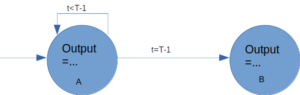
The machine must stay in state ‘A’ during ‘T’ clock periods, moving then to state ‘B’.

Because the timer’s initial value is zero, it must count from 0 to ‘T’ - 1 in order to span ‘T’ clock cycles.

Let us consider a case, where we are in state ‘A’, but due to some reason, ‘t’ overshoots, abruptly, i.e., ‘t’ > ‘T’ - 1, to a random big value, or this happened, due to some reset glitch, in the counter. The state diagram fails here because it needs to move to state ‘B’, when ‘t’ > ‘T’ - 1, as per our problem statement, not just when it is ‘T’ - 1, as is specified in the state diagram above. This has happened due to an incomplete understanding of the problem statement, leading to underspecification.

It should be noted here that, there is more than one concept being covered here implicitly in the aforementioned example, but attention needs to be drawn to the value which is being plugged in here by chance, or should we say randomly, to a certain extent. It was not really expected while designing the solution, which in turn led us to discover chinks in our logic armor.

When we are using a verification environment based in Python, random values could be provided in a user-defined manner, using its useful pseudo-random number library. Most pseudo-random number generators (PRNGs) are built on algorithms involving some kind of recursive method starting from a base value that is determined by an input called the seed.

The seeding of the Random Number Generator in Python must be performed explicitly in one point in our code via the seed() method.

Here, some of the functions are listed to get started with them, for verification purposes.

• randint(a, b) and randrange(start, stop, step) produce a random value within a specified range, equivalent to SystemVerilog $urandom_range().
• getrandbits(k) produces a random number of length k bits.
• choice(seq) or choices(seq, weights) chooses an item from a sequence {list}, the latter implements a weighted choice – seq can be a list of anything you like {ints, classes, functions...}
• shuffle(seq) randomly reorders a list (in place).
• sample(seq, k) returns a sequence of k items from ‘seq’ chosen at random.

To understand their implementation and for other important information, kindly refer to this link.

The verification domain can get computationally intensive, and involves the usage of probability, statistics, and discrete mathematics, along with intuition and a knack for exploration.

“When n bugs are detected and rectified, doesn’t mean the design is bug-free,  it means n bugs less in the final product ”

So, to get to something near to a bug-free design - we use verification tools (like Vyoma’s UpTickPro which is being used during the verification hackathon - CTB) that can automatically give input and check for proper output and return a summary of the test. Now the verifier writes in a file the possible inputs and expected output. The tool will take up the design in HDL and provide input as mentioned and compare the output with the expected one and return a summary of the testing.

Join us to explore such concepts and more, where we use Python to leverage its library-rich environment feasible for verification using Vyoma’s UpTickPro platform, in this edition of Capture the Bug hackathon, organized by NIELIT, Calicut, mentored by IIT Madras, in association with VLSI System Design and Vyoma Systems.

Hackathon details - https://nielithackathon.in/