You see how every sentence in the title is connected!!!
As you are aware about the big launch on “CCS Library” course, I just wanted to bring one thing over here for you to think about. Its ‘Scaling’. We are moving from 180nm to 45nm to 7nm. Let’s take an example of 180nm and 45nm. That’s a scaling factor of 0.25 (this can be debated as 45nm/180nm will give 0.25 and vice-versa will give 4. Let’s stick to former i.e 0.25).
Now, there are tons of scaling mechanisms, like short wire, long wire, constant thickness, etc. For this discussion, let’s stick to full scaling for long wires, as shown in below image:
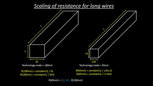
This is rather a shocking observation, and in great contrast with gate delay. Gate delay reduces year by year, whereas delay of long wires goes up by 6.25% (i.e. by a factor of sqr(0.25) = 0.0625). That’s huge!!
Let’s demo both wires in SPICE. So here we will model the wire as distributed RC network, and plot the output response V(wire_out) with step pulse as input V(out), as shown in below image. Ignore the naming convention as the course is in continuation with STA-1, STA-2, Circuit design and SPICE simulations. Do not forget to finish these courses 100% before even registering to “CCS timing” course
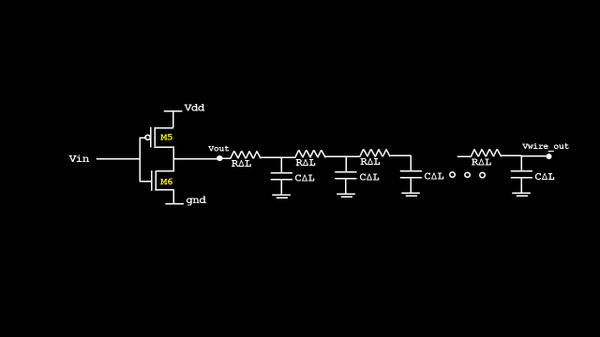
Be aware, that the problem statement here is the inverter has to drive the long wire in both technology nodes, while giving an accurate response at Vwire_out.
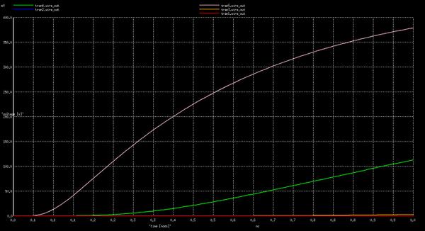
Assume wire length to be 50m. So, if we pluck out the wire from the above network, keep reducing the wire size by half, and just SPICE it with 180nm technology node for all wire lengths, assuming R∆L as 75K and C∆L as 100pF (taken default values from ngspice), it gives us the below response
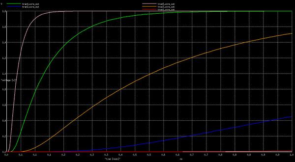
To interpret above, the bottom red line is the Vwire_out response for 50m wire, blue line is for 25m, and finally white line is for 3.125m. This can be (simply) interpreted, that, at 180nm technology node, a wire length of 3.125m can be driven by CMOS network
But, when we scale down in the way we shown above in first image i.e. by a factor of 0.25, we need to scale up the resistance by (1/S2) and so now the R∆L becomes (75K/sqr[0.25]) = 1200K, and let’s draw a similar step response of wire at 45nm, it looks something like below image:
Now, previous driver models for inverters i.e. thevenin or Norton model were good to express various timing arcs using output capacitance only. But they are not efficient enough to drive a high impedance network as shown above. Solution – CCS timing
Just try to solve thevenin voltage divider circuit, and you would get to know that output will just follow input voltage, which is not accurate. No issues, if you find it difficult to do so, I will be making it simpler in my course
Next step is to plot the inverter response to these high impedance network. And that’s even more interesting. Let’s keep that for next blog or for the course.
Just as Albert Einstein said “Any fool can make things bigger, more complex and more violent. It takes a touch of genius – and a lot of courage – to move in the opposite direction”
Be a genius, and wait for my CCS timing course. Till then please complete 100% the necessary courses (STA-1, STA-2, Circuit design and SPICE simulations Part 1 and 2).
But please be aware of the concepts, and I will make this course a smooth and happy journey for you. Happy Learning!!